
2.3.1 Spline Based Shapes


|
2.3 Advanced Features |
POV-Ray 3.6 for UNIX documentation 2.3.1 Spline Based Shapes |
2.3.2 Polygon Based Shapes |

|
After we have gained some experience with the simpler shapes available in POV-Ray it is time to go on to the more advanced, thrilling shapes.
We should be aware that the shapes described in this and the following two chapters are not trivial to understand. We need not be worried though if we do not know how to use them or how they work. We just try the examples and play with the features described in the reference chapter. There is nothing better than learning by doing.
You may wish to skip to the chapter "Simple Texture Options" before proceeding with these advanced shapes.
In the real world, lathe refers to a process of making patterned
rounded shapes by spinning the source material in place and carving pieces out as it turns. The results can be
elaborate, smoothly rounded, elegant looking artefacts such as table legs, pottery, etc. In POV-Ray, a lathe object is
used for creating much the same kind of items, although we are referring to the object itself rather than the means of
production.
Here is some source for a really basic lathe.
  #include "colors.inc"
  background{White}
  camera {
    angle 10
    location <1, 9, -50>
    look_at <0, 2, 0>
  }
  light_source {
    <20, 20, -20> color White
  }
  lathe {
    linear_spline
    6,
    <0,0>, <1,1>, <3,2>, <2,3>, <2,4>, <0,4>
    pigment { Blue }
    finish {
      ambient .3
      phong .75
    }
  }
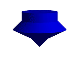
We render this, and what we see is a fairly simply type of lathe, which looks like a child's top. Let's take a look at how this code produced the effect.
First, a set of six points is declared which the raytracer connects with lines. We note that there are only two components in the vectors which describe these points. The lines that are drawn are assumed to be in the x-y-plane, therefore it is as if all the z-components were assumed to be zero. The use of a two-dimensional vector is mandatory (Attempting to use a 3D vector would trigger an error... with one exception, which we will explore later in the discussion of splines).
Once the lines are determined, the ray-tracer rotates this line around the y-axis, and we can imagine a trail being left through space as it goes, with the surface of that trail being the surface of our object.
The specified points are connected with straight lines because we used the linear_spline keyword.
There are other types of splines available with the lathe, which will result in smooth curving lines, and even rounded
curving points of transition, but we will get back to that in a moment.
First, we would like to digress a moment to talk about the difference between a lathe and a surface of revolution object (SOR). The SOR object, described in a separate tutorial, may seem terribly similar to the lathe at first glance. It too declares a series of points and connects them with curving lines and then rotates them around the y-axis. The lathe has certain advantages, such as different kinds of splines, linear, quadratic and cubic, and one more thing:
The simpler mathematics used by a SOR does not allow the curve to double back over the same y-coordinates, thus, if using a SOR, any sudden twist which cuts back down over the same heights that the curve previously covered will trigger an error. For example, suppose we wanted a lathe to arc up from <0,0> to <2,2>, then to dip back down to <4,0>. Rotated around the y-axis, this would produce something like a gelatin mold - a rounded semi torus, hollow in the middle. But with the SOR, as soon as the curve doubled back on itself in the y-direction, it would become an illegal declaration.
Still, the SOR has one powerful strong point: because it uses simpler order mathematics, it generally tends to render faster than an equivalent lathe. So in the end, it is a matter of: we use a SOR if its limitations will allow, but when we need a more flexible shape, we go with the lathe instead.
It would be helpful, in order to understand splines, if we had a sort of Spline Workshop where we could practice manipulating types and points of splines and see what the effects were like. So let's make one! Now that we know how to create a basic lathe, it will be easy:
#include "colors.inc"
  camera {
    orthographic
    up <0, 5, 0>
    right <5, 0, 0>
    location <2.5, 2.5, -100>
    look_at <2.5, 2.5, 0>
  }
  /* set the control points to be used */
  #declare Red_Point    = <1.00, 0.00>;
  #declare Orange_Point = <1.75, 1.00>;
  #declare Yellow_Point = <2.50, 2.00>;
  #declare Green_Point  = <2.00, 3.00>;
  #declare Blue_Point   = <1.50, 4.00>;
  /* make the control points visible */
  cylinder { Red_Point, Red_Point - <0,0,20>, .1
    pigment { Red }
    finish { ambient 1 }
  }
  cylinder { Orange_Point, Orange_Point - <0,0,20>, .1
    pigment { Orange }
    finish { ambient 1 }
  }
  cylinder { Yellow_Point, Yellow_Point - <0,0,20>, .1
    pigment { Yellow }
    finish { ambient 1 }
  }
  cylinder { Green_Point, Green_Point - <0,0,20>, .1
    pigment { Green }
    finish { ambient 1 }
  }
  cylinder { Blue_Point, Blue_Point- <0,0,20>, .1
    pigment { Blue }
    finish { ambient 1 }
  }
  /* something to make the curve show up */
  lathe {
    linear_spline
    5,
    Red_Point,
    Orange_Point,
    Yellow_Point,
    Green_Point,
    Blue_Point
    pigment { White }
    finish { ambient 1 }
  }
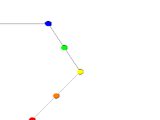
Now, we take a deep breath. We know that all looks a bit weird, but with some simple explanations, we can easily see what all this does.
First, we are using the orthographic camera. If we have not read up on that yet, a quick summary is: it renders the
scene flat, eliminating perspective distortion so that in a side view, the objects look like they were drawn
on a piece of graph paper (like in the side view of a modeler or CAD package). There are several uses for this
practical new type of camera, but here it is allowing us to see our lathe and cylinders edge on, so that what
we see is almost like a cross section of the curve which makes the lathe, rather than the lathe itself. To further
that effect, we eliminated shadowing with the ambient 1 finish, which of course also eliminates the need
for lighting. We have also positioned this particular side view so that <0,0> appears at the lower left of our
scene.
Next, we declared a set of points. We note that we used 3D vectors for these points rather than the 2D vectors we expect in a lathe. That is the exception we mentioned earlier. When we declare a 3D point, then use it in a lathe, the lathe only uses the first two components of the vector, and whatever is in the third component is simply ignored. This is handy here, since it makes this example possible.
Next we do two things with the declared points. First we use them to place small diameter cylinders at the locations of the points with the circular caps facing the camera. Then we re-use those same vectors to determine the lathe.
Since trying to declare a 2D vector can have some odd results, and is not really what our cylinder declarations need anyway, we can take advantage of the lathe's tendency to ignore the third component by just setting the z-coordinate in these 3D vectors to zero.
The end result is: when we render this code, we see a white lathe against a black background showing us how the
curve we have declared looks, and the circular ends of the cylinders show us where along the x-y-plane our control
points are. In this case, it is very simple. The linear spline has been used so our curve is just straight lines
zig-zagging between the points. We change the declarations of Red_Point and Blue_Point to
read as follows.
  #declare Red_Point  = <2.00, 0.00>;
  #declare Blue_Point = <0.00, 4.00>;
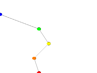
We re-render and, as we can see, all that happens is that the straight line segments just move to accommodate the new position of the red and blue points. Linear splines are so simple, we could manipulate them in our sleep, no?
Let's try something different. First, we change the points to the following.
  #declare Red_Point    = <1.00, 0.00>;
  #declare Orange_Point = <2.00, 1.00>;
  #declare Yellow_Point = <3.50, 2.00>;
  #declare Green_Point  = <2.00, 3.00>;
  #declare Blue_Point   = <1.50, 4.00>;
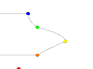
We then go down to the lathe declaration and change linear_spline to quadratic_spline. We
re-render and what do we have? Well, there is a couple of things worthy of note this time. First, we will see that
instead of straight lines we have smooth arcs connecting the points. These arcs are made from quadratic curves, so our
lathe looks much more interesting this time. Also, Red_Point is no longer connected to the curve. What
happened?
Well, while any two points can determine a straight line, it takes three to determine a quadratic curve. POV-Ray looks not only to the two points to be connected, but to the point immediately preceding them to determine the formula of the quadratic curve that will be used to connect them. The problem comes in at the beginning of the curve. Beyond the first point in the curve there is no previous point. So we need to declare one. Therefore, when using a quadratic spline, we must remember that the first point we specify is only there so that POV-Ray can determine what curve to connect the first two points with. It will not show up as part of the actual curve.
There is just one more thing about this lathe example. Even though our curve is now put together with smooth curving lines, the transitions between those lines is... well, kind of choppy, no? This curve looks like the lines between each individual point have been terribly mismatched. Depending on what we are trying to make, this could be acceptable, or, we might long for a more smoothly curving shape. Fortunately, if the latter is true, we have another option.
The quadratic spline takes longer to render than a linear spline. The math is more complex. Taking longer still is
the cubic spline, yet for a really smoothed out shape this is the only way to go. We go back into our example, and
simply replace quadratic_spline with cubic_spline. We render one more time, and take a look
at what we have.
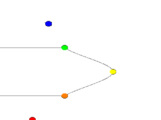
While a quadratic spline takes three points to determine the curve, a cubic needs four. So, as we might expect, Blue_Point
has now dropped out of the curve, just as Red_Point did, as the first and last points of our curve are
now only control points for shaping the curves between the remaining points. But look at the transition from
Orange_Point to Yellow_Point and then back to Green_Point. Now, rather than looking
mismatched, our curve segments look like one smoothly joined curve.
finally there is another kind of quadratic spline, the bezier_spline. This one takes four points per
section. The start point, the end points and in between, two control points. To use it, we will have to make a few
changes to our work shop. Delete the Yellow point, delete the Yellow cylinder. Change the points to:
  #declare Red_Point    = <2.00, 1.00>;
  #declare Orange_Point = <3.00, 1.50>;
  #declare Green_Point  = <3.00, 3.50>;
  #declare Blue_Point   = <2.00, 4.00>;
And change the lathe to:
  lathe {
    bezier_spline
    4,
    Red_Point,
    Orange_Point,
    Green_Point,
    Blue_Point
    pigment { White }
    finish { ambient 1 }
  }
The, green and orange, control points are not connected to the curve. Move them around a bit, for example #declare
Orange_Point = <1.00, 1.50>;. The line that can be drawn from the start point to its closest control
point (red to orange) shows the tangent of the curve at the start point. Same for the end point, blue to green.
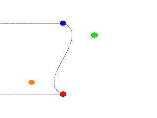
One spline segment is nice, two is nicer. So we will add another segment and connect it to the blue point. One segment has four points, so two segments have eight. The first point of the second segment is the same as the last point of the first segment. The blue point. So we only have to declare three more points. Also we have to move the camera a bit and add more cylinders. Here is the complete scene again:
#include "colors.inc"
camera {
orthographic
up <0, 7, 0>
right <7, 0, 0>
location <3.5, 4, -100>
look_at <3.5, 4, 0>
}
/* set the control points to be used */
#declare Red_Point = <2.00, 1.00>;
#declare
 Orange_Point = <1.00, 1.50>;
#declare Green_Point = <3.00, 3.50>;
#declare Blue_Point = <2.00, 4.00>;
#declare Green_Point2 = <3.00, 4.50>;
#declare Orange_Point2= <1.00, 6.50>;
#declare Red_Point2 = <2.00, 7.00>;
/* make the control points visible */
cylinder { Red_Point, Red_Point - <0,0,20>, .1
pigment { Red } finish { ambient 1 }
}
cylinder { Orange_Point, Orange_Point - <0,0,20>, .1
pigment { Orange } finish { ambient 1 }
}
cylinder { Green_Point, Green_Point - <0,0,20>, .1
pigment { Green } finish { ambient 1 }
}
cylinder { Blue_Point, Blue_Point- <0,0,20>, .1
pigment { Blue } finish { ambient 1 }
}
cylinder { Green_Point2, Green_Point2 - <0,0,20>, .1
pigment { Green } finish { ambient 1 }
}
cylinder { Orange_Point2, Orange_Point2 - <0,0,20>, .1
pigment { Orange } finish { ambient 1 }
}
cylinder { Red_Point2, Red_Point2 - <0,0,20>, .1
pigment { Red } finish { ambient 1 }
}
/* something to make the curve show up */
lathe {
bezier_spline
8,
Red_Point, Orange_Point, Green_Point, Blue_Point
Blue_Point, Green_Point2, Orange_Point2, Red_Point2
pigment { White }
finish { ambient 1 }
}
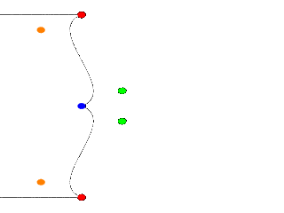
A nice curve, but what if we want a smooth curve? Let us have a look at the tangents on the Blue_point, draw the
lines Green_Point, Blue_point and Green_Point2, Blue_point. Look at the angle they make, it is as sharp as the dent in
the curve. What if we make the angle bigger? What if we make the angle 180�? Try a few positions for Green_point2 and
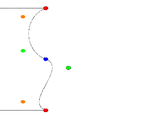
end with #declare Green_Point2 = <1.00, 4.50>;. A smooth curve. If we make sure that the two
control points and the connection point are on one line, the curve is perfectly smooth. In general this can be
achieved by #declare Green_Point2 = Blue_Point+(Blue_Point-Green_Point);
The concept of splines is a handy and necessary one, which will be seen again in the prism and polygon objects. But with a little tinkering we can quickly get a feel for working with them.
Bottles, vases and glasses make nice objects in ray-traced scenes. We want to create a golden cup using the surface of revolution object (SOR object).
We first start by thinking about the shape of the final object. It is quite difficult to come up with a set of points that describe a given curve without the help of a modeling program supporting POV-Ray's surface of revolution object. If such a program is available we should take advantage of it.
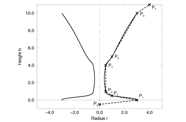
We will use the point configuration shown in the figure above. There are eight points describing the curve that will be rotated about the y-axis to get our cup. The curve was calculated using the method described in the reference section (see "Surface of Revolution").
Now it is time to come up with a scene that uses the above SOR object. We create a file called sordemo.pov
and enter the following text.
  #include "colors.inc"
  #include "golds.inc"
  camera {
    location <10, 15, -20>
    look_at <0, 5, 0>
    angle 45
  }
  background { color rgb<0.2, 0.4, 0.8>  }
  light_source { <100, 100, -100> color rgb 1 }
  plane {
    y, 0
    pigment { checker color Red, color Green scale 10 }
  }
  sor {
    8,
    <0.0,  -0.5>,
    <3.0,   0.0>,
    <1.0,   0.2>,
    <0.5,   0.4>,
    <0.5,   4.0>,
    <1.0,   5.0>,
    <3.0,  10.0>,
    <4.0,  11.0>
    open
    texture { T_Gold_1B }
  }
The scene contains our cup object resting on a checkered plane. Tracing this scene results in the image below.
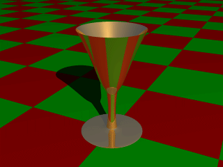
The surface of revolution is described by starting with the number of points followed by the points. Points from second to last but one are listed with ascending heights. Each of them determines the radius of the curve for a given height. E. g. the first valid point (second listed) tells POV-Ray that at height 0.0 the radius is 3. We should take care that each point has a larger height than its predecessor. If this is not the case the program will abort with an error message. First and last point from the list are used to determine slope at beginning and end of curve and can be defined for any height.
The prism is essentially a polygon or closed curve which is swept along a linear path. We can imagine the shape so
swept leaving a trail in space, and the surface of that trail is the surface of our prism. The curve or polygon making
up a prism's face can be a composite of any number of sub-shapes, can use any kind of three different splines, and can
either keep a constant width as it is swept, or slowly tapering off to a fine point on one end. But before this gets
too confusing, let's start one step at a time with the simplest form of prism. We enter and render the following POV
code (see file prismdm1.pov).
  #include "colors.inc"
  background{White}
  camera {
    angle 20
    location <2, 10, -30>
    look_at <0, 1, 0>
  }
  light_source { <20, 20, -20> color White }
  prism {
    linear_sweep
    linear_spline
    0, // sweep the following shape from here ...
    1, // ... up through here
    7, // the number of points making up the shape ...
    <3,5>, <-3,5>, <-5,0>, <-3,-5>, <3, -5>, <5,0>, <3,5>
    pigment { Green }
  }
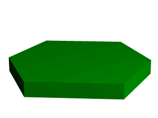
This produces a hexagonal polygon, which is then swept from y=0 through y=1. In other words, we now have an extruded hexagon. One point to note is that although this is a six sided figure, we have used a total of seven points. That is because the polygon is supposed to be a closed shape, which we do here by making the final point the same as the first. Technically, with linear polygons, if we did not do this, POV-Ray would automatically join the two ends with a line to force it to close, although a warning would be issued. However, this only works with linear splines, so we must not get too casual about those warning messages!
If we followed the section on splines covered under the lathe tutorial (see section "Understanding The Concept of Splines"), we know that there are two additional kinds of splines besides linear: the quadratic and the cubic spline. Sure enough, we can use these with prisms to make a more free form, smoothly curving type of prism.
There is just one catch, and we should read this section carefully to keep from tearing our hair out over mysterious "too few points in prism" messages which keep our prism from rendering. We can probably guess where this is heading: how to close a non-linear spline. Unlike the linear spline, which simply draws a line between the last and first points if we forget to make the last point equal to the first, quadratic and cubic splines are a little more fussy.
First of all, we remember that quadratic splines determine the equation of the curve which connects any two points based on those two points and the previous point, so the first point in any quadratic spline is just control point and will not actually be part of the curve. What this means is: when we make our shape out of a quadratic spline, we must match the second point to the last, since the first point is not on the curve - it is just a control point needed for computational purposes.
Likewise, cubic splines need both the first and last points to be control points, therefore, to close a shape made with a cubic spline, we must match the second point to the second from last point. If we do not match the correct points on a quadratic or cubic shape, that is when we will get the "too few points in prism" error. POV-Ray is still waiting for us to close the shape, and when it runs out of points without seeing the closure, an error is issued.
Confused? Okay, how about an example? We replace the prism in our last bit of code with this one (see file prismdm2.pov).
  prism {
    cubic_spline
    0, // sweep the following shape from here ...
    1, // ... up through here
    6, // the number of points making up the shape ...
    < 3, -5>, // point#1 (control point... not on curve)
    < 3,  5>, // point#2  ... THIS POINT ...
    <-5,  0>, // point#3
    < 3, -5>, // point#4
    < 3,  5>, // point#5 ... MUST MATCH THIS POINT
    <-5,  0>  // point#6 (control point... not on curve)
    pigment { Green }
  }
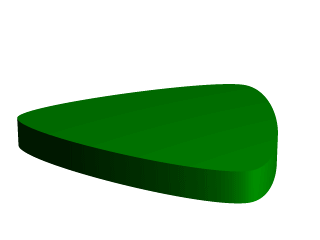
This simple prism produces what looks like an extruded triangle with its corners sanded smoothly off. Points two, three and four are the corners of the triangle and point five closes the shape by returning to the location of point two. As for points one and six, they are our control points, and are not part of the shape - they are just there to help compute what curves to use between the other points.
Now a handy thing to note is that we have made point one equal point four, and also point six equals point three.
Yes, this is important. Although this prism would still be legally closed if the control points were not what we have
made them, the curve transitions between points would not be as smooth. We change points one and six to <4,6>
and <0,7> respectively and re-render to see how the back edge of the shape is altered (see file prismdm3.pov).
To put this more generally, if we want a smooth closure on a cubic spline, we make the first control point equal to the third from last point, and the last control point equal to the third point. On a quadratic spline, the trick is similar, but since only the first point is a control point, make that equal to the second from last point.
Just as with the polygon object (see section "Polygon Object") the
prism is very flexible, and allows us to make one prism out of several sub-prisms. To do this, all we need to do is
keep listing points after we have already closed the first shape. The second shape can be simply an add on going off
in another direction from the first, but one of the more interesting features is that if any even number of sub-shapes
overlap, that region where they overlap behaves as though it has been cut away from both sub-shapes. Let's look at
another example. Once again, same basic code as before for camera, light and so forth, but we substitute this complex
prism (see file prismdm4.pov).
  prism {
    linear_sweep
    cubic_spline
    0,  // sweep the following shape from here ...
    1,  // ... up through here
    18, // the number of points making up the shape ...
    <3,-5>, <3,5>, <-5,0>, <3, -5>, <3,5>, <-5,0>,//sub-shape #1
    <2,-4>, <2,4>, <-4,0>, <2,-4>, <2,4>, <-4,0>, //sub-shape #2
    <1,-3>, <1,3>, <-3,0>, <1, -3>, <1,3>, <-3,0> //sub-shape #3
    pigment { Green }
  }
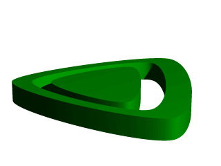
For readability purposes, we have started a new line every time we moved on to a new sub-shape, but the ray-tracer of course tells where each shape ends based on whether the shape has been closed (as described earlier). We render this new prism, and look what we have got. It is the same familiar shape, but it now looks like a smaller version of the shape has been carved out of the center, then the carved piece was sanded down even smaller and set back in the hole.
Simply, the outer rim is where only sub-shape one exists, then the carved out part is where sub-shapes one and two overlap. In the extreme center, the object reappears because sub-shapes one, two, and three overlap, returning us to an odd number of overlapping pieces. Using this technique we could make any number of extremely complex prism shapes!
In our original prism, the keyword linear_sweep is actually optional. This is the default sweep
assumed for a prism if no type of sweep is specified. But there is another, extremely useful kind of sweep: the conic
sweep. The basic idea is like the original prism, except that while we are sweeping the shape from the first height
through the second height, we are constantly expanding it from a single point until, at the second height, the shape
has expanded to the original points we made it from. To give a small idea of what such effects are good for, we
replace our existing prism with this (see file prismdm4.pov):
  prism {
    conic_sweep
    linear_spline
    0, // height 1
    1, // height 2
    5, // the number of points making up the shape...
    <4,4>,<-4,4>,<-4,-4>,<4,-4>,<4,4>
    rotate <180, 0, 0>
    translate <0, 1, 0>
    scale <1, 4, 1>
    pigment { gradient y scale .2 }
  }
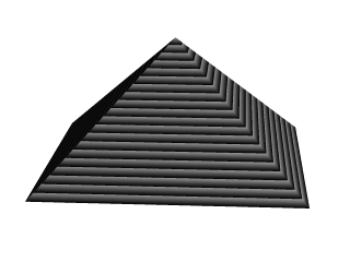
The gradient pigment was selected to give some definition to our object without having to fix the lights and the camera angle right at this moment, but when we render it, what have we created? A horizontally striped pyramid! By now we can recognize the linear spline connecting the four points of a square, and the familiar final point which is there to close the spline.
Notice all the transformations in the object declaration. That is going to take a little explanation. The rotate and translate are easy. Normally, a conic sweep starts full sized at the top, and tapers to a point at y=0, but of course that would be upside down if we are making a pyramid. So we flip the shape around the x-axis to put it right side up, then since we actually orbited around the point, we translate back up to put it in the same position it was in when we started.
The scale is to put the proportions right for this example. The base is eight units by eight units, but the height (from y=1 to y=0) is only one unit, so we have stretched it out a little. At this point, we are probably thinking, "why not just sweep up from y=0 to y=4 and avoid this whole scaling thing?"
That is a very important gotcha! with conic sweeps. To see what is wrong with that, let's try and put it into
practice (see file prismdm5.pov). We must make sure to remove the scale statement, and then replace the
line which reads
1, // height 2
with
4, // height 2
This sets the second height at y=4, so let's re-render and see if the effect is the same.
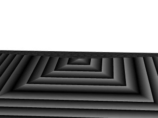
Whoa! Our height is correct, but our pyramid's base is now huge! What went wrong here? Simple. The base, as we described it with the points we used actually occurs at y=1 no matter what we set the second height for. But if we do set the second height higher than one, once the sweep passes y=1, it keeps expanding outward along the same lines as it followed to our original base, making the actual base bigger and bigger as it goes.
To avoid losing control of a conic sweep prism, it is usually best to let the second height stay at y=1, and use a scale statement to adjust the height from its unit size. This way we can always be sure the base's corners remain where we think they are.
That leads to one more interesting thing about conic sweeps. What if we for some reason do not want them to taper all the way to a point? What if instead of a complete pyramid, we want more of a ziggurat step? Easily done. After putting the second height back to one, and replacing our scale statement, we change the line which reads
0, // height 1
to
0.251, // height 1
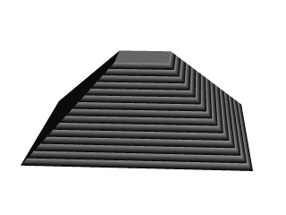
When we re-render, we see that the sweep stops short of going all the way to its point, giving us a pyramid without a cap. Exactly how much of the cap is cut off depends on how close the first height is to the second height.
A Sphere Sweep Object is the space a sphere occupies during its movement along a spline.
So we need to specify
the kind of spline we want and a list of control points to define that spline. To help POV-Ray we tell how many
control points will be used. In addition, we also define the radius the moving sphere should have when passing through
each of these control points.
The syntax of the sphere_sweep object is:
  sphere_sweep {
    linear_spline | b_spline | cubic_spline
    NUM_OF_SPHERES,

    CENTER, RADIUS,
    CENTER, RADIUS,
    ...
    CENTER, RADIUS
    [tolerance DEPTH_TOLERANCE]
    [OBJECT_MODIFIERS]
  }
An example for a linear Sphere Sweep would be:
  sphere_sweep {
    linear_spline
    4,
    <-5, -5, 0>, 1
    <-5,  5, 0>, 1
    < 5, -5, 0>, 1
    < 5,  5, 0>, 1
  }
This object is described by four spheres. You can use as many spheres as you like to describe the object, but you will need at least two spheres for a linear Sphere Sweep, and four spheres for one approximated with a cubic_spline or b_spline.
The example above would result in an object shaped like the letter "N". The sphere sweep goes through all points which are connected with straight cones.
Changing the kind of interpolation to a cubic_spline produces a quite different, slightly bent, object. It then starts at the second sphere and ends at the last but one. Since the first and last points are used to control the spline, you need two more points to get a shape that can be compared to the linear sweep. Let's add them:
  sphere_sweep {
    cubic_spline
    6,
    <-4, -5, 0>, 1
    <-5, -5, 0>, 1
    <-5,  5, 0>, 0.5
    < 5, -5, 0>, 0.5
    < 5,  5, 0>, 1
    < 4,  5, 0>, 1
    tolerance 0.1
 }
So the cubic sweep creates a smooth sphere sweep actually going through all points (except the first and last one). In this example the radius of the second and third spheres have been changed. We also added the "tolerance" keyword, because dark spots appeared on the surface with the default value (0.000001).
When using a b_spline, the resulting object is somewhat similar to the cubic sweep, but does not actually go through the control points. It lies somewhere between them.
Bicubic patches are useful surface representations because they allow an easy definition of surfaces using only a few control points. The control points serve to determine the shape of the patch. Instead of defining the vertices of triangles, we simply give the coordinates of the control points. A single patch has 16 control points, one at each corner, and the rest positioned to divide the patch into smaller sections. POV-Ray does not ray trace the patches directly, they are approximated using triangles as described in the Scene Description Language section.
Bicubic patches are almost always created by using a third party modeler, but for this tutorial we will manipulate
them by hand. Modelers that support Bicubic patches and export to POV-Ray can be found in the links
collection on our server
Let's set up a basic scene and start exploring the Bicubic patch.
#version 3.5;
global_settings {assumed_gamma 1.0}
background {rgb <1,0.9,0.9>}
camera {location <1.6,5,-6> look_at <1.5,0,1.5> angle 40}
light_source {<500,500,-500> rgb 1 }

#declare B11=<0,0,3>; #declare B12=<1,0,3>; //
#declare B13=<2,0,3>; #declare B14=<3,0,3>; // row 1

#declare B21=<0,0,2>; #declare B22=<1,0,2>; //
#declare B23=<2,0,2>; #declare B24=<3,0,2>; // row 2

#declare B31=<0,0,1>; #declare B32=<1,0,1>; //
#declare B33=<2,0,1>; #declare B34=<3,0,1>; // row 3

#declare B41=<0,0,0>; #declare B42=<1,0,0>; //
#declare B43=<2,0,0>; #declare B44=<3,0,0>; // row 4

bicubic_patch {
   type 1 flatness 0.001
   u_steps 4 v_steps 4
   uv_vectors
   <0,0> <1,0> <1,1> <0,1>
   B11, B12, B13, B14
   B21, B22, B23, B24
   B31, B32, B33, B34
   B41, B42, B43, B44
   uv_mapping
   texture {
      pigment {
         checker
         color rgbf <1,1,1,0.5>
         color rgbf <0,0,1,0.7>
         scale 1/3
      }
      finish {phong 0.6 phong_size 20}
   }
   no_shadow
}
The points B11, B14, B41, B44 are the corner points of the patch. All other points are control points. The names of the declared points are as follows: B for the colour of the patch, the first digit gives the row number, the second digit the column number. If you render the above scene, you will get a blue & white checkered square, not very exciting. First we will add some spheres to make the control points visible. As we do not want to type the code for 16 spheres, we will use an array and a while loop to construct the spheres.
#declare Points=array[16]{
   B11, B12, B13, B14
   B21, B22, B23, B24
   B31, B32, B33, B34
   B41, B42, B43, B44
}
#declare I=0;
#while (I<16)
   sphere {
      Points[I],0.1
      no_shadow
      pigment{
         #if (I=0|I=3|I=12|I=15)
            color rgb <1,0,0>
         #else
            color rgb <0,1,1>
         #end
      }
   }
   #declare I=I+1;
#end
Rendering this scene will show the patch with its corner points in red and its control points in cyan. Now it is
time to start exploring.
Change B41 to <-1,0,0> and render.
Change B41 to <-1,1,0>
and render.
Change B41 to < 1,2,1> and render.
Let's do some exercise with the control points. Start with a flat patch again.
Change B42 to <1,2,0>
and B43 to <2,-2,0> and render.
Change B42 and B43 back to their original positions and try B34
to <4,2,1> and B24 to <2,-2,2> and render. Move the points around some more,
also try the control points in the middle.
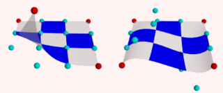
After all this we notice two things:
Now go back to our spline work shop and have a look at the bezier_spline again. Indeed, the points B11,B12,B13,B14, make up a bezier_spline. So do the points B11,B21,B31,B41 and B41,B42,B43,B44 and B14,B24,B34,B44.
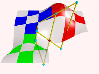
So far we have only been looking at one single patch, but one of the strengths of the Bicubic patch lays in the fact that they can be connected smoothly, to form bigger shapes. The process of connecting is relatively simple as there are actually only two rules to follow. It can be done by using a well set up set of macros or by using a modeler. To give an idea what is needed we will do a simple example by hand.
First put the patch in our scene back to its flat position. Then change #declare B14 = <3,0,3>;
#declare B24 = <3,2,2>; #declare B34 = <3.5,1,1> ; #declare B44 = <3,-1,0>; #declare B41 =
<0,-1,0>; Move the camera a bit back camera { location <3.1,7,-8> look_at <3,-2,1.5>
angle 40 } and delete all the code for the spheres. We will now try and stitch a patch to the right side of the
current one. Off course the points on the left side (column 1) of the new patch have to be in the same position as the
points on the right side (column 4) of the blue one.
Render the scene, including our new patch:
#declare R11=B14; #declare R12=<4,0,3>;     //
#declare R13=<5,0,3>; #declare R14=<6,0,3>; // row 1

#declare R21=B24; #declare R22=<4,0,2>;     //
#declare R23=<5,0,2>; #declare R24=<6,0,2>; // row 2

#declare R31=B34; #declare R32=<4,0,1>;     //
#declare R33=<5,0,1>; #declare R34=<6,0,1>; // row 3

#declare R41=B44; #declare R42=<4,0,0>;     //
#declare R43=<5,0,0>; #declare R44=<6,0,0>; // row 4

bicubic_patch {
   type 1 flatness 0.001
   u_steps 4 v_steps 4
   uv_vectors
   <0,0> <1,0> <1,1> <0,1>
   R11, R12, R13, R14
   R21, R22, R23, R24
   R31, R32, R33, R34
   R41, R42, R43, R44
   uv_mapping
   texture {
      pigment {
         checker
         color rgbf <1,1,1,0.5>
         color rgbf <1,0,0,0.7>
         scale 1/3
      }
      finish {phong 0.6 phong_size 20}
   }
   no_shadow
}
This is a rather disappointing result. The patches are connected, but not exactly smooth. In connecting patches the same principles apply as for connecting two 2D bezier splines as we see in the spline workshop. Control point, connection point and the next control point should be on one line to give a smooth result. Also it is preferred, not required, that the distances from both control points to the connection point are the same. For the Bicubic patch we have to do the same, for all connection points involved in the joint. So, in our case, the following points should be on one line:
To achieve this we do:
#declare R12=B14+(B14-B13);
#declare R22=B24+(B24-B23);
#declare R32=B34+(B34-B33);
#declare R42=B44+(B44-B43);

This renders a smooth surface. Adding a third patch in front is relative simple now:
#declare G11=B41;      #declare G12=B42;                //
#declare G13=B43;      #declare G14=B44;                // row 1

#declare G21=B41+(B41-B31); #declare G22=B42+(B42-B32); //
#declare G23=B43+(B43-B33); #declare G24=B44+(B44-B34); // row 2

#declare G31=<0,0,-2>; #declare G32=<1,0,-2>;           //
#declare G33=<2,0,-2>; #declare G34=<3,2,-2>;           // row 3

#declare G41=<0,0,-3>; #declare G42=<1,0,-3>;           //
#declare G43=<2,0,-3>; #declare G44=<3,0,-3>            // row 4

bicubic_patch {
   type 1 flatness 0.001
   u_steps 4 v_steps 4
   uv_vectors
   <0,0> <1,0> <1,1> <0,1>
   G11, G12, G13, G14
   G21, G22, G23, G24
   G31, G32, G33, G34
   G41, G42, G43, G44
   uv_mapping
   texture {
      pigment {
         checker
         color rgbf <1,1,1,0.5>
         color rgbf <0,1,0,0.7>
         scale 1/3
      }
      finish {phong 0.6 phong_size 20}
   }
   no_shadow
}
Finally, let's put a few spheres back in the scene and add some cylinders to visualize what is going on. See what happens if you move for example B44, B43, B33 or B34.
#declare Points=array[8]{B33,B34,R32,B43,B44,R42,G23,G24}
#declare I=0;
#while (I<8)
   sphere {
      Points[I],0.1
      no_shadow
      pigment{
         #if (I=4)
            color rgb <1,0,0>
         #else
            color rgb <0,1,1>
         #end
      }
   }
   #declare I=I+1;
#end
union {
   cylinder {B33,B34,0.04} cylinder {B34,R32,0.04}
   cylinder {B43,B44,0.04} cylinder {B44,R42,0.04}
   cylinder {G23,G24,0.04}
   cylinder {B33,B43,0.04} cylinder {B43,G23,0.04}
   cylinder {B34,B44,0.04} cylinder {B44,G24,0.04}
   cylinder {R32,R42,0.04}
   no_shadow
   pigment {color rgb <1,1,0>}
}
The hard part in using the Bicubic patch is not in connecting several patches. The difficulty is keeping control over the shape you want to build. As patches are added, in order to keep the result smooth, control over the position of many points gets restrained.
The text object is a primitive that can use TrueType fonts and TrueType Collections to create text
objects. These objects can be used in CSG, transformed and textured just like any other POV primitive.
For this tutorial, we will make two uses of the text object. First, let's just make some block letters sitting on a
checkered plane. Any TTF font should do, but for this tutorial, we will use the timrom.ttf or cyrvetic.ttf
which come bundled with POV-Ray.
We create a file called textdemo.pov and edit it as follows:
  #include "colors.inc"
  camera {
    location <0, 1, -10>
    look_at 0
    angle 35
  }
  light_source { <500,500,-1000> White }
  plane {
    y,0
    pigment { checker Green White }
  }
Now let's add the text object. We will use the font timrom.ttf and we will create the string
"POV-RAY 3.0". For now, we will just make the letters red. The syntax is very simple. The first string in
quotes is the font name, the second one is the string to be rendered. The two floats are the thickness and offset
values. The thickness float determines how thick the block letters will be. Values of .5 to 2 are usually best for
this. The offset value will add to the kerning distance of the letters. We will leave this a 0 for now.
  text {
    ttf "timrom.ttf" "POV-RAY 3.0" 1, 0
    pigment { Red }
  }
Rendering this at 200x150 -A, we notice that the letters are off to the right of the screen. This is
because they are placed so that the lower left front corner of the first letter is at the origin. To center the string
we need to translate it -x some distance. But how far? In the docs we see that the letters are all 0.5 to 0.75 units
high. If we assume that each one takes about 0.5 units of space on the x-axis, this means that the string is about 6
units long (12 characters and spaces). Let's translate the string 3 units along the negative x-axis.
  text {
    ttf "timrom.ttf" "POV-RAY 3.0" 1, 0
    pigment { Red }
    translate -3*x
  }
That is better. Now let's play around with some of the parameters of the text object. First, let's raise the thickness float to something outlandish... say 25!
  text {
    ttf "timrom.ttf" "POV-RAY 3.0" 25, 0
    pigment { Red }
    translate -2.25*x
  }
Actually, that is kind of cool. Now let's return the thickness value to 1 and try a different offset value. Change the offset float from 0 to 0.1 and render it again.
Wait a minute?! The letters go wandering off up at an angle! That is not what the docs describe! It almost looks as
if the offset value applies in both the x- and y-axis instead of just the x axis like we intended. Could it be that a
vector is called for here instead of a float? Let's try it. We replace 0.1 with 0.1*x and
render it again.
That works! The letters are still in a straight line along the x-axis, just a little further apart. Let's verify
this and try to offset just in the y-axis. We replace 0.1*x with 0.1*y. Again, this works
as expected with the letters going up to the right at an angle with no additional distance added along the x-axis. Now
let's try the z-axis. We replace 0.1*y with 0.1*z. Rendering this yields a disappointment.
No offset occurs! The offset value can only be applied in the x- and y-directions.
Let's finish our scene by giving a fancier texture to the block letters, using that cool large thickness value, and
adding a slight y-offset. For fun, we will throw in a sky sphere, dandy up our plane a bit, and use a little more
interesting camera viewpoint (we render the following scene at 640x480 +A0.2):
  #include "colors.inc"
  camera {
    location <-5,.15,-2>
    look_at <.3,.2,1>
    angle 35
  }
  light_source { <500,500,-1000> White }
  plane {
    y,0
    texture {
      pigment { SeaGreen }
      finish { reflection .35 specular 1 }
      normal { ripples .35 turbulence .5 scale .25 }
    }
  }
  text {
    ttf "timrom.ttf" "POV-RAY 3.0" 25, 0.1*y
    pigment { BrightGold }
    finish { reflection .25 specular 1 }
    translate -3*x
  }
  #include "skies.inc"
  sky_sphere { S_Cloud5 }
Let's try using text in a CSG object. We will attempt to create an inlay in a stone block using a text object. We
create a new file called textcsg.pov and edit it as follows:
  #include "colors.inc"
  #include "stones.inc"
  background { color rgb 1 }
  camera {
    location <-3, 5, -15>
    look_at 0
    angle 25
  }
  light_source { <500,500,-1000> White }
Now let's create the block. We want it to be about eight units across because our text string "POV-RAY 3.0" is about six units long. We also want it about four units high and about one unit deep. But we need to avoid a potential coincident surface with the text object so we will make the first z-coordinate 0.1 instead of 0. Finally, we will give this block a nice stone texture.
  box {
    <-3.5, -1, 0.1>, <3.5, 1, 1>
    texture { T_Stone10 }
  }
Next, we want to make the text object. We can use the same object we used in the first tutorial except we will use slightly different thickness and offset values.
  text {
    ttf "timrom.ttf" "POV-RAY 3.0" 0.15, 0
    pigment { BrightGold }
    finish { reflection .25 specular 1 }
    translate -3*x
  }
We remember that the text object is placed by default so that its front surface lies directly on the x-y-plane. If the front of the box begins at z=0.1 and thickness is set at 0.15, the depth of the inlay will be 0.05 units. We place a difference block around the two objects.
  difference {
    box {
      <-3.5, -1, 0.1>, <3.5, 1, 1>
      texture { T_Stone10 }
    }
    text {
      ttf "timrom.ttf" "POV-RAY 3.0" 0.15, 0
      pigment { BrightGold }
      finish { reflection .25 specular 1 }
      translate -3*x
    }
  }
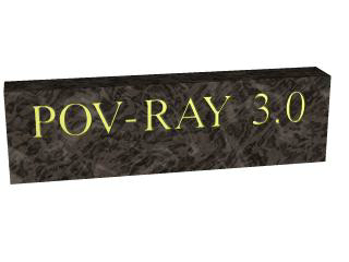
We render this at 200x150 -A. We can see the inlay clearly and that it is indeed a bright gold color.
We re-render at 640x480 +A0.2 to see the results more clearly, but be forewarned... this trace will take
a little time.

|
2.3 Advanced Features | 2.3.1 Spline Based Shapes | 2.3.2 Polygon Based Shapes |

|